Graphics: MATLAB plots with LaTeX-formatted labels

For graphic designers, creating visuals is natural, whereas for people working with computation and modelling, it is a separate challenge.

I approach this through coding:

• plots are created in MATLAB and Python (Matplotlib),
• the LaTeX interpreter is used to keep text formatting consistent with the document,
• drawings are created in TikZ (a LaTeX package for electrical and block diagrams).

This approach provides high-quality graphics with mathematical notation and a script-based workflow.

In this post, I show a minimal MATLAB example that includes all key elements in a single figure. Examples in Python and TikZ will be covered separately.

Somewhat more advanced figures include multi-panel layouts (using subplot function), inset plots, dual axes (left and right Y-axes), and more advanced formatting. These will be described in separate posts.

Damped oscillatory waveform in MATLAB

Below is an example plot exported as a PNG image for use in a document.

The plotted function is:

\[i(t)=I_\mathrm{m}\cos(\omega t)\,\mathrm{e}^{-t/\tau},\]

where: $I_\mathrm{m} = 1$ – peak amplitude [p.u.],
$f = 50$ – frequency [Hz],
$\omega = 2\pi f$ – angular frequency [rad/s],
$\tau = 0.05$ – time constant [s].

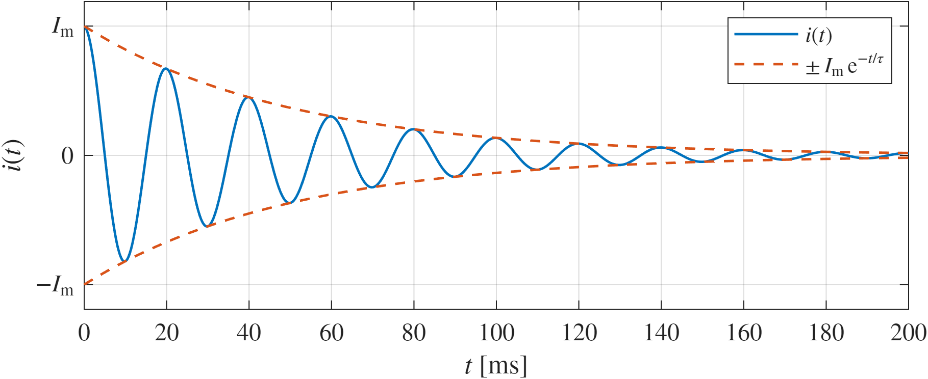Fig. 1. Damped oscillatory waveform.

Files used in this example:

• MATLAB source file (.m),
• output (PNG),
• output (PDF).

MATLAB code

An example including the key elements: waveform, envelope, axis labels, and legend.

Key setting: LaTeX interpreter as default for all text elements.

The description is provided directly in code comments.

%% MATLAB settings
clc; clear; format compact;

%% Graphics settings
% Use LaTeX for axis labels, text, and legend
set(groot, ...
    'defaultAxesTickLabelInterpreter','latex', ...
    'defaultTextInterpreter','latex', ...
    'defaultLegendInterpreter','latex');

% Global graphics defaults for consistent appearance
set(groot, ...
    'defaultLineLineWidth',1.15, ...
    'defaultAxesFontSize',12, ...
    'defaultTextFontSize',12);

% Figure size: [left, bottom, width, height] in points
set(gcf, 'Units', 'points', 'Position', [200,150,500,200]);

%% Signal parameters
% Cosine current with exponentially decaying amplitude
Im  = 1;          % peak current amplitude
f   = 50;         % frequency [Hz]
w   = 2*pi*f;     % angular frequency [rad/s]
tau = 0.05;       % time constant [s]

%% Time vector and waveform definition
% Signal computed over 1 s
t = 0:1e-4:1;     

% Damped oscillatory current waveform
i = Im*cos(w*t).*exp(-t/tau);

% Positive exponential envelope
envelope = Im*exp(-t/tau);

%% Plot
% Color definitions
blueColor = [0.0000 0.4470 0.7410];
redColor  = [0.8500 0.3250 0.0980];

% Plot with handles
hp1 = plot(t, i, 'Color', blueColor); hold on; grid on;
hp2 = plot(t, envelope, '--', t, -envelope, '--');
set(hp2, 'Color', redColor);
hold off;

%% Axes limits
xlim([0 200]*1e-3); % Only initial transient part is displayed, 0-200 ms
ylim(1.19*[-1 1]);  % Approximately 1.2

%% Axis ticks and labels
% Time axis in milliseconds for easier interpretation
xtick_values = 0:20e-3:200e-3;
xticks(xtick_values);
xticklabels(num2str(xtick_values'*1e3));
xlabel('$t\:[\mathrm{ms}]$');

% Y-axis normalized to peak current Im
yticks([-1 0 1]);
yticklabels({'$-I_\mathrm{m}$','0','$I_\mathrm{m}$'});
ylabel('$i(t)$');

%% Title and legend
title('$i(t)=I_\mathrm{m}\cos(\omega t)\,\mathrm{e}^{-t/\tau}$');

legend([hp1 hp2(1)], ...
    {'$i(t)$', '$\pm\,I_\mathrm{m}\,\mathrm{e}^{-t/\tau}$'}, ...
    'Location','northeast');

%% Export figure
% PDF (vector graphics) – suitable for LaTeX documents
exportgraphics(gcf, 'current_oscillatory_waveform.pdf');

% PNG (raster graphics) – suitable for web use
exportgraphics(gcf, 'current_oscillatory_waveform.png', 'Resolution', 300);

Default MATLAB color palette (RGB)

The file with the default MATLAB color palette is available here (it is useful to have it at hand when creating plots).

Code snippet:

%% MATLAB default color order (RGB)
% Order matches MATLAB default axes ColorOrder

blueColor       = [0.0000 0.4470 0.7410]; % blue
redColor        = [0.8500 0.3250 0.0980]; % red
yellowColor     = [0.9290 0.6940 0.1250]; % yellow
purpleColor     = [0.4940 0.1840 0.5560]; % purple
greenColor      = [0.4660 0.6740 0.1880]; % green
lightBlueColor  = [0.3010 0.7450 0.9330]; % light blue
darkRedColor    = [0.6350 0.0780 0.1840]; % dark red

These colors are used by MATLAB by default for successive data series.

Example plot:

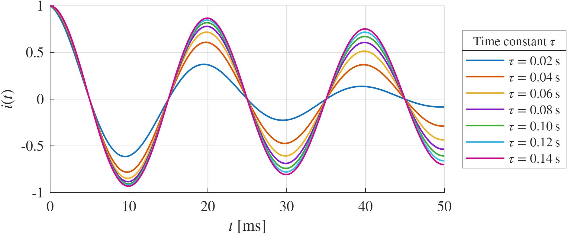Fig. 2. Damped oscillatory waveforms for different time constants.

Notes

• The LaTeX interpreter in MATLAB supports only a subset of LaTeX.
• It is useful to export plots to PDF (vector) in addition to PNG.

Summary

A script-based approach provides reproducible and high-quality plots.

Code → plot → have fun.