Graphics: TikZ in LaTeX – basics and first circuit (circuitikz)

TikZ is a LaTeX package for creating graphics. A drawing is described by code, not inserted as an image.

This approach gives good control over details, consistency with the document (e.g. fonts), and easy modifications later (edit the code and recompile).

In this post I show the basics of TikZ: from a simple example to a first electrical circuit in circuitikz.

Target drawing shown in this post:

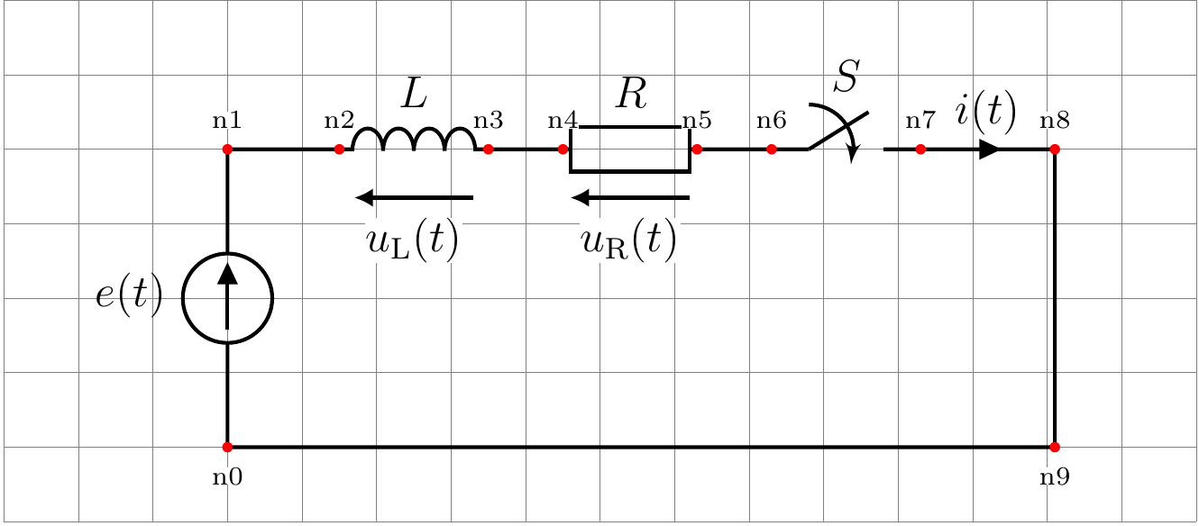Fig. 1. Example TikZ drawing with grid and nodes.

---

Minimal example – circle

A TikZ drawing is a piece of code inside the tikzpicture environment.

Example circle with center, radius and diameter:

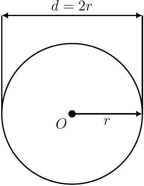Fig. 2. Example TikZ circle.

Code:

\begin{tikzpicture}[scale=2]
    % circle
    \draw (0,0) circle (1);
    % center
    \fill (0,0) circle (1.5pt) node[below left] {$O$};
    % radius
    \draw[->] (0,0) -- (1,0) node[midway, below] {$r$};
    % extension lines
    \draw (-1,0) -- (-1,1.4);
    \draw (1,0) -- (1,1.4);
    % diameter (dimension line)
    \draw[<->] (-1,1.4) -- (1,1.4)
    node[midway, above] {$d=2r$};
\end{tikzpicture}

Basic elements:

• \begin{tikzpicture} – drawing environment
• \draw – drawing
• (x,y) – coordinates
• -- – segment
• node – label
• [->], [<->] – arrows

---

RLC circuit in TikZ (circuitikz)

Below is the RLC circuit shown in three variants: from simple to more advanced.

Variant 1

Simplest version. Short code, but arrows are not aligned horizontally.

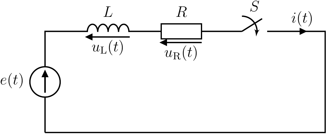Fig. 3. RLC circuit without grid and nodes.

Code:

\begin{circuitikz}[scale=0.7,line width=1pt]
    \draw
    (0,0) to[isource, l=$e(t)$] (0,4)
    -- (1.5,4)
    to[L, l=$L$, v_<=$u_\mathrm{L}(t)$] (3.5,4)
    -- (4.5,4)
    to[R, l=$R$, v_<=$u_\mathrm{R}(t)$] (6.3,4)
    -- (7.3,4)
    to[closing switch, l=$S$, bipoles/length=2cm] (9.3,4)
    to[short, i>^=$i(t)$] (11.1,4)
    -- (11.1,0) -- (0,0);
\end{circuitikz}

Variant 2

Same circuit, using relative coordinates (++).

\begin{circuitikz}[scale=0.7,line width=1pt]
    \draw
    (0,0) to[isource, l=$e(t)$] ++(0,4)
    -- ++(1.5,0)
    to[L, l=$L$, v_<=$u_\mathrm{L}(t)$] ++(2.0,0)
    -- ++(1.0,0)
    to[R, l=$R$, v_<=$u_\mathrm{R}(t)$] ++(1.8,0)
    -- ++(1.0,0)
    to[closing switch, l=$S$, bipoles/length=2cm] ++(2.0,0)
    to[short, i>^=$i(t)$] ++(1.8,0)
    -- ++(0,-4) -- ++(-11.1,0);
\end{circuitikz}

Variant 3

Final version. More code, but full control and aligned arrows.

Fig. 4. RLC circuit with grid and nodes.

Grid and nodes can be disabled:

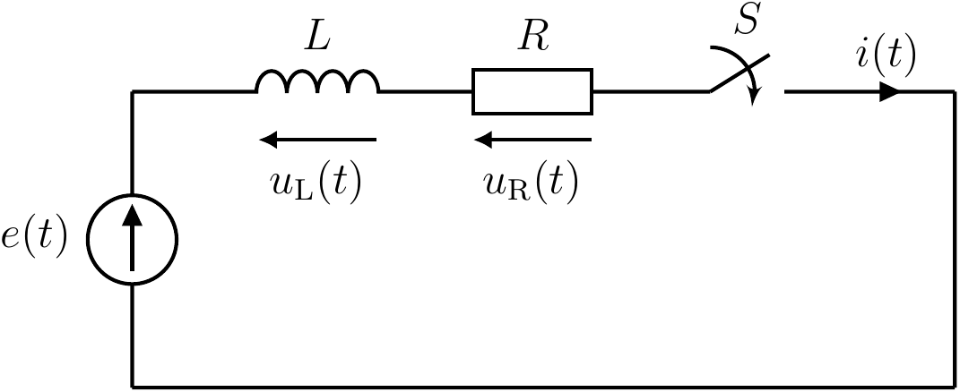Fig. 5. Final RLC circuit.

Code:

\begin{circuitikz}[scale=0.7,line width=1pt]
	% --- Debug switches ---
	% Enable or disable auxiliary drawing elements (grid and nodes)
		
	\newif\ifshowgrid   % Controls visibility of the background grid
	\newif\ifshownodes  % Controls visibility of debug nodes and labels
		
	\showgridtrue      % Set to \showgridtrue to show the grid
	\shownodestrue      % Set to \shownodesfalse to hide debug markers and labels
		
	% Debug grid to assist with manual layout alignment
	\ifshowgrid
	\draw [help lines] (-3,-1) grid (13,6);
	\fi
		
	% --- Point definitions ---
	\coordinate (n0) at (0,0);
	\coordinate (n1) at (0,4);
	\coordinate (n2) at (1.5,4);
	\coordinate (n3) at (3.5,4);
	\coordinate (n4) at (4.5,4);
	\coordinate (n5) at (6.3,4);
	\coordinate (n6) at (7.3,4);
	\coordinate (n7) at (9.3,4);
	\coordinate (n8) at (11.1,4);
	\coordinate (n9) at (11.1,0);
		
	% Consistent style for debug labels
	\tikzset{
		debug label/.style={
			font=\scriptsize,
			fill=white,
			inner sep=0pt
		}
	}
		
	% --- Main circuit ---
	\draw
	(n0) to[isource, l=$e(t)$] (n1)
	(n1) to[short, -] (n2)
	(n2) to[L=$L$] (n3)
	(n3) to[short, -] (n4)
	(n4) to[R=$R$] (n5)
	(n5) to[short, -] (n6)
	(n6) to[/tikz/circuitikz/bipoles/length=2cm, closing switch=$S$] (n7)
	(n7) to[short, -, i>^=$i(t)$] (n8)
	(n8) to[short, -] (n9)
	(n9) to[short, -] (n0)
	;
		
	% --- Manually drawn voltage arrows ---
	% NOTE: Voltage arrows are drawn manually to control length and alignment
	
	% --- arrow length ---
	\def\varrow{1.6}  % total length
		
	% u_L
	\draw[<-]
	($(n2)!0.5!(n3)+(-0.5*\varrow,-0.65)$) --
	($(n2)!0.5!(n3)+(0.5*\varrow,-0.65)$)
	node[midway, below=5pt, fill=white, inner sep=0pt] {$u_\mathrm{L}(t)$};
		
	% u_R
	\draw[<-]
	($(n4)!0.5!(n5)+(-0.5*\varrow,-0.65)$) --
	($(n4)!0.5!(n5)+(0.5*\varrow,-0.65)$)
	node[midway, below=5pt, fill=white, inner sep=0pt] {$u_\mathrm{R}(t)$};		
	
	% --- Debug: point names ---
	\ifshownodes
		\foreach \p in {n1,n2,n3,n4,n5,n6,n7,n8}{
			\fill[red] (\p) circle (2pt);
			\node[above=5pt, debug label] at (\p) {\p};
		}
		\foreach \p in {n0,n9}{
			\fill[red] (\p) circle (2pt);
			\node[below=5pt, debug label] at (\p) {\p};
		}
	\fi
\end{circuitikz}

Summary

TikZ allows drawings to be defined directly in LaTeX as code. This gives full control and easy modifications.

You can start with simple examples and then move to more complex drawings like circuits in circuitikz.